10. スライディングモード制御器の設計
スライディングモード制御則の設計の目的は、切換面にない状態から切換面に収束させて、その面上に状態を保つことである。これを保証することは制御器の設計にかかっている。ここでは、式(1)に示す\(m\)個の入力を有する線形な系にたいして、スライディングモードを生じさせることを考える。$$\begin{cases} \dot x = A x + B u \\ \sigma = S x = 0 \end{cases} \;\;\; \cdots (1)$$制御入力は、式(2)のように切り換えるものとする。$$ u = \begin{cases} u^{+} & \text{if} \quad \sigma \gt 0 \\ u^{-} & \text{if} \quad \sigma \lt 0 \end{cases} \;\;\; \cdots (2)$$この\(u\)について検討する。
対角化法による設計
対角化法の目的は、多入力系を\(m\)個の1入力系のスライディングモードに分解して、見通しの良い制御則を設計することにある。このとき、スライディングモードの存在条件は、式(3)で与えられる。$$\lim_{t \to \infty} \sigma_i \dot \sigma_i \lt 0 \quad (i = 1,2, \cdots , m) \;\;\; \cdots (3)$$式(2)の制御入力に対して、ある正則変換\(Q^{-1}(x,t) S(x) B\)を適用すると、制御入力は、式(4)で表せる。$$u^{*} = Q^{-1}(x,t) S(x) B u \;\;\; \cdots (4)$$但し、\(S = \partial \sigma / \partial x,\quad \det(SB) \neq 0\)とする。行列\(Q(x,t)\)は、\(m \times m\)の任意な対角行列である。$$Q(x,t) = \text{diag}[q_1, q_2, \cdots , q_m]$$式(1)に式(4)を使うと、$$\dot x = A x + B(SB)^{-1} Q u^{*}$$ となる。また、$$\dot \sigma = S \dot x = S A x + Q u^{*} \;\;\; \cdots (5)$$を得る。式(5)によって、制御則\(u_i^{*+}, u_i^{*-}\)を$$\begin{cases} q_i(x,t)u_i^{*+} \lt -\text{grad}\{\sigma_i(x)\}Ax = -\sum_{j=1}^n S_{ij}A_j x & \text{if} \quad \sigma_i(x) \gt 0 \\ q_i(x,t)u_i^{*-} \gt -\text{grad}\{\sigma_i(x)\}Ax = -\sum_{j=1}^n S_{ij}A_j x & \text{if} \quad \sigma_i(x) \lt 0 \end{cases} \;\;\; \cdots (6)$$のように選べば、スライディングモードの存在条件の式(3)を満たす。式(6)の条件が\(\sigma = 0\)の近傍だけでなく、\([x_1,x_2, \cdots , x_n]\)の全領域で成立すれば、同時に到達条件を満足する。このとき実際の制御入力は、式(7)で与えられる。$$u = (SB)^{-1}Q(x,t)u^{*} \;\;\; \cdots (7)$$
Pythonによるシミュレーション例
2入力2状態システム \((n=2, m=2)\)を対象としたシミュレーション例を示す。状態方程式:\(\dot x = Ax + Bu \)、状態ベクトル: \(x = [x_1, x_2]^T \)、制御入力ベクトル: \(u = [u_1, u_2]^T \)とする。ここで、$$A = \begin{bmatrix} 0 & 1 \\ -1 & -1 \end{bmatrix} \quad \quad B = \begin{bmatrix} 0 & 1 \\ 1 & 1 \end{bmatrix}$$である。また、\(\sigma = Sx\)において、$$S = \begin{bmatrix} 1 & 1 \\ -1 & 1 \end{bmatrix}$$とする。このとき、$$SB = \begin{bmatrix} 1 & 1 \\ -1 & 1 \end{bmatrix} \begin{bmatrix} 0 & 1 \\ 1 & 1 \end{bmatrix} = \begin{bmatrix} 1 & 2 \\ 1 & 0 \end{bmatrix}$$となる。 \(\det(SB) = -2 \neq 0\) なので、$$(SB)^{-1} = \begin{bmatrix} 0 & 1 \\ 0.5 & -0.5 \end{bmatrix}$$である。また、$$Q = \begin{bmatrix} 1 & 0 \\ 0 & 1 \end{bmatrix}$$とする。なお、式(6)を満たす一般的な制御則として、次のような形が用いられる。 $$q_i u_i^∗=−(S A x)_i − \eta_i \text{sgn}(\sigma_i) \quad (\eta_i > 0) $$ ここで、 \(\text{sgn}(\cdot)\) は符号関数である。もし \(\sigma_i > 0\) ならば \(q_i u_i^* = -(SAx)_i - \eta_i < -(SAx)_i \)であり、 もし \(\sigma_i < 0\) ならば \(q_i u_i^* = -(SAx)_i + \eta_i > -(SAx)_i \)となるので、式(6)の条件を満たす。
図1(上)は、状態変数の時間応答 (\(x_1(t), x_2(t)\))である。 初期状態 \([3.0, 1.0]^T\) から、制御により状態変数が時間とともに変化し、最終的には原点 \([0,0]^T\) に収束している。図1(下)は、切換変数の時間応答 (\(\sigma_1(t), \sigma_2(t)\))である。\(\sigma_1 = x_1 + x_2\) と \(\sigma_2 = -x_1 + x_2\) で定義されるスライディング変数が、初期値から急速に0に近づき、0近傍に留まる(スライディングモードが達成された)様子が分かる。図2(上)は、位相面軌跡(\(x_1-x_2\) 平面)である。状態軌跡が初期点から開始し、スライディング平面 \(\sigma_1=0\) (直線 \(x_2 = -x_1\)) および \(\sigma_2=0\) (直線 \(x_2 = x_1\)) の両方、あるいはそれらの交点(原点)に向かって運動する様子が分かる。システムの状態は、まずどちらかのスライディング平面に到達し、その後は両方の平面が交差する原点へと収束していく。図2(下)は、制御入力の時間応答 (\(u_1(t), u_2(t)\))である。スライディング変数が0でない間(到達位相)は、状態をスライディング平面に拘束するために制御入力が変化する。スライディングモードに入った後は、外乱やモデル化誤差がなければ、状態を平面上に維持するための等価制御入力となる。
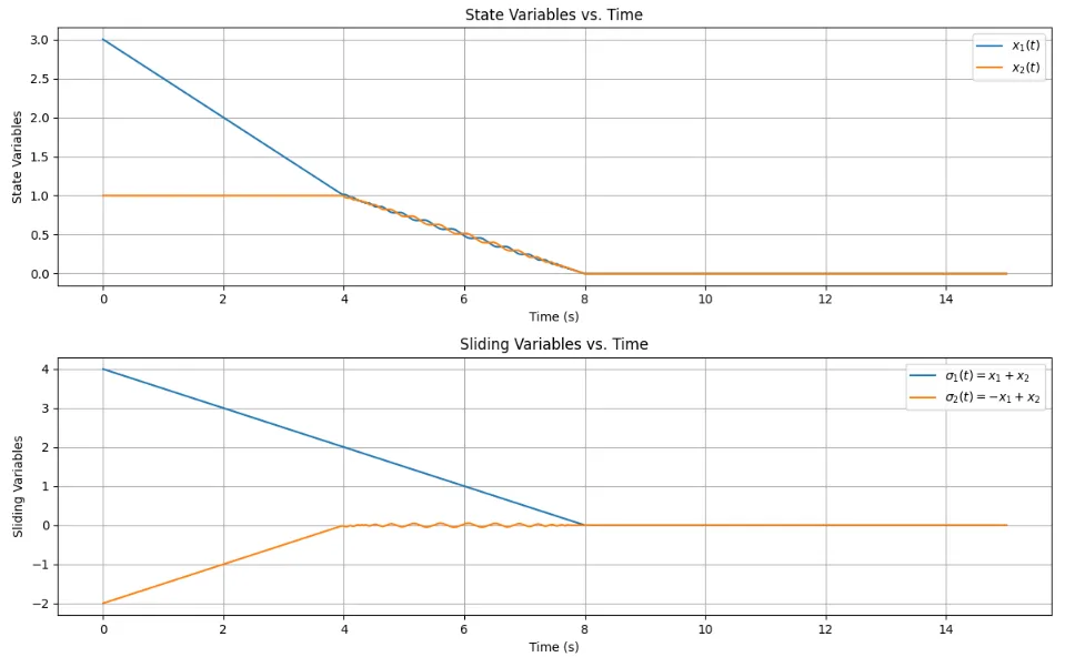
切換変数\(\sigma_1, \sigma_2\)の時間応答(下)
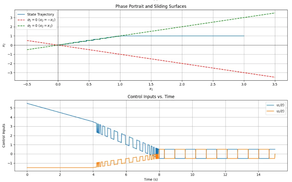
制御入力\(u_1,u_2\)の時間応答(下)
import numpy as np
from scipy.integrate import solve_ivp
import matplotlib.pyplot as plt
# --- System Parameters ---
# A Matrix
A = np.array([[0, 1],
[-1, -1]])
# B Matrix
B = np.array([[0, 1],
[1, 1]])
# --- Sliding Mode Control Parameters ---
# S Matrix (defines sliding surface sigma = Sx)
S = np.array([[1, 1],
[-1, 1]])
# Calculate SB and (SB)^-1
SB = S @ B
if np.linalg.det(SB) == 0:
raise ValueError("det(SB) is zero. Choose S and B appropriately.")
SB_inv = np.linalg.inv(SB)
# Q Matrix (Diagonal, q_i > 0)
Q = np.diag([1.0, 1.0]) # q1 = 1, q2 = 1
# Control design parameters (eta_i > 0 for reaching law)
eta = np.array([0.5, 0.5]) # eta1, eta2
# --- Simulation Parameters ---
x0 = np.array([3.0, 1.0]) # Initial state
t_span = (0, 15) # Simulation time span (seconds)
t_eval = np.linspace(t_span[0], t_span[1], 1000) # Time points for evaluation
# --- Define the System Dynamics for ODE Solver ---
def system_dynamics(t, x):
# Calculate sliding variable sigma = Sx
sigma_val = S @ x # m x 1 vector
# Calculate SAx
SAx = S @ A @ x # m x 1 vector
# Calculate u_star (element-wise)
u_star = np.zeros_like(sigma_val) # m x 1 vector
for i in range(len(sigma_val)):
# q_i * u_star_i = -(SAx)_i - eta_i * sgn(sigma_i)
# u_star_i = (1/q_i) * (-(SAx)_i - eta_i * sgn(sigma_i))
if Q[i, i] == 0: # Should not happen for a valid Q
raise ValueError(f"Q[{i},{i}] is zero.")
sign_sigma_i = np.sign(sigma_val[i])
# If sigma_i = 0, np.sign(0) = 0.
# Theoretically, the inequality holds for sigma_i != 0.
# For chattering reduction, a saturation function can be used instead of sgn.
# Here, the simple sign function is used.
u_star[i] = (1 / Q[i, i]) * (-SAx[i] - eta[i] * sign_sigma_i)
# Calculate actual control input u
# u = (SB)^-1 * Q * u_star
u = SB_inv @ Q @ u_star # m x 1 vector
# System dynamics: dx/dt = Ax + Bu
dxdt = A @ x + B @ u
return dxdt
# --- Solve the ODE using a numerical integrator ---
sol = solve_ivp(system_dynamics, t_span, x0, t_eval=t_eval, method='RK45')
# --- Extract Results ---
t = sol.t
x_res = sol.y
# Calculate sliding variable sigma over time for plotting
sigma_res = np.array([S @ x_col for x_col in x_res.T]).T
# --- Plot Results ---
plt.rc('font', family='sans-serif') # Fallback font
plt.figure(figsize=(12, 15))
# Plot state variables
plt.subplot(4, 1, 1)
plt.plot(t, x_res[0, :], label='$x_1(t)$')
plt.plot(t, x_res[1, :], label='$x_2(t)$')
plt.title('State Variables vs. Time')
plt.xlabel('Time (s)')
plt.ylabel('State Variables')
plt.legend()
plt.grid(True)
# Plot sliding variables
plt.subplot(4, 1, 2)
plt.plot(t, sigma_res[0, :], label='$\sigma_1(t) = x_1 + x_2$')
plt.plot(t, sigma_res[1, :], label='$\sigma_2(t) = -x_1 + x_2$')
plt.title('Sliding Variables vs. Time')
plt.xlabel('Time (s)')
plt.ylabel('Sliding Variables')
plt.legend()
plt.grid(True)
# Plot phase portrait and sliding surfaces
plt.subplot(4, 1, 3)
plt.plot(x_res[0, :], x_res[1, :], label='State Trajectory')
# Sliding surfaces: sigma_1 = x1 + x2 = 0 => x2 = -x1
# sigma_2 = -x1 + x2 = 0 => x2 = x1
x1_plot = np.linspace(np.min(x_res[0, :]) - 0.5, np.max(x_res[0, :]) + 0.5, 100)
if S[0,1] != 0: # s12
x2_sigma1_zero = -(S[0,0]/S[0,1]) * x1_plot # x2 = -(s11/s12)*x1
plt.plot(x1_plot, x2_sigma1_zero, 'r--', label='$\sigma_1=0$ ($x_2 = -x_1$)')
if S[1,1] != 0: # s22
x2_sigma2_zero = -(S[1,0]/S[1,1]) * x1_plot # x2 = -(s21/s22)*x1
plt.plot(x1_plot, x2_sigma2_zero, 'g--', label='$\sigma_2=0$ ($x_2 = x_1$)')
plt.title('Phase Portrait and Sliding Surfaces')
plt.xlabel('$x_1$')
plt.ylabel('$x_2$')
plt.axhline(0, color='black', linewidth=0.5)
plt.axvline(0, color='black', linewidth=0.5)
plt.legend()
plt.grid(True)
# plt.axis('equal') # Adjust as needed
# Re-calculate and plot control inputs
u_res_list = []
for i in range(len(t)):
xi = x_res[:, i]
sigma_val_i = S @ xi
SAx_i = S @ A @ xi
u_star_i_vec = np.zeros_like(sigma_val_i)
for j in range(len(sigma_val_i)):
sign_sigma_ij = np.sign(sigma_val_i[j])
u_star_i_vec[j] = (1 / Q[j,j]) * (-SAx_i[j] - eta[j] * sign_sigma_ij)
u_i_vec = SB_inv @ Q @ u_star_i_vec
u_res_list.append(u_i_vec)
u_res = np.array(u_res_list).T
plt.subplot(4, 1, 4)
plt.plot(t, u_res[0, :], label='$u_1(t)$')
plt.plot(t, u_res[1, :], label='$u_2(t)$')
plt.title('Control Inputs vs. Time')
plt.xlabel('Time (s)')
plt.ylabel('Control Inputs')
plt.legend()
plt.grid(True)
plt.tight_layout()
plt.show()
三次の線形系への適用例
三次の線形系でスライディングモード制御を考える。$$ \dot x = A x + B u \\ A = \begin{bmatrix} 0 & 1 & 0 \\ 0 & 0 & 1 \\ -1 & -2 & -3 \end{bmatrix}, \quad B = \begin{bmatrix} 0 & 0 \\ 0 & 1 \\ 1 & 0 \end{bmatrix}$$切換超平面を以下とする。$$\sigma(x) = S x = \begin{bmatrix} 33 & 1.2 & 14 \\ 400 & 40 & 1.2 \end{bmatrix} \begin{bmatrix} x_1 \\ x_2 \\ x_3 \end{bmatrix} = \begin{bmatrix} 0 \\ 0 \end{bmatrix}$$ \(Q=I\)とすると、新しい制御入力は、$$u^* = Q^{-1} S B u = S B u = K x$$と書ける。この\(u^*\)は状態フィードバックの形で与えられるとしている。つまり、$$u^* = \begin{bmatrix} u_1^* \\ u_2^* \end{bmatrix} = K x = \begin{bmatrix} k_{11} & k_{12} & k_{13} \\ k_{21} & k_{22} & k_{23} \end{bmatrix} \begin{bmatrix} x_1 \\ x_2 \\ x_3 \end{bmatrix}$$である。ただし、$$k_{ij} = \begin{cases} k_{ij}^+ & \text{if} \;\; \sigma_i x_j \gt 0 \\ k_{ij}^- & \text{if} \;\; \sigma_i x_j \lt 0 \end{cases}$$また、$$\dot \sigma = S \dot x = S A x + u^* = \begin{bmatrix} \dot \sigma_1 \\ \dot \sigma_2 \end{bmatrix} = S A x + \begin{bmatrix} u_1^* \\ u_2^* \end{bmatrix}$$を得る。各成分について書くと、$$\dot \sigma_i = (S A x)_i + u_i^* = (S A x)_i + \sum_{j=1}^3 k_{ij} x_j \quad (i=1,2)$$である。スライディングモードが存在するための条件(到達条件)は、\(\sigma_i\)に対して$$\sigma_i \dot \sigma_i \lt 0 \quad (for\; \sigma_i \neq 0)$$なので、$$\sigma_i \left( (S A x)_i + \sum_{j=1}^3 k_{ij} x_j \right) \lt 0$$となる。これにより、\(\sigma_i \dot \sigma_i \lt 0\)を保証するように\(k_{ij}^+,\; k_{ij}^-\)を選定する。従って、実際の制御入力は、$$u = (SB)^{-1}u^* = (SB)^{-1}\begin{bmatrix} k_{11} & k_{12} & k_{13} \\ k_{21} & k_{22} & k_{23} \end{bmatrix} x$$と表せる。