7. 切換超平面の設計（1）

連続時間系のスライディングモード制御における切換超平面の設計を考える。

極配置による設計法

式(1)の線形時不変系で考える。 $$\dot x_a = A x_a + B u \;\;\; \cdots (1)$$ ここで、$x_a \in R^n,\; u \in R^m$で、$(A,\;B)$は可制御とする。このときの拘束条件$\sigma_i = 0 ,\; (i=1,2, \cdots, m)$の集合を $$\sigma = S x_a = 0 \;\;\; \cdots (2)$$ と与える。 正準系への座標変換$x_a = T x$により、式(1)、式(2)のシステムは、 $$\begin{cases} \dot x_1 = A_{11}x_1 + A_{12} x_2 \\ \dot x_2 = A_{21} x_1 + A_{22} x_2 + B_2 u \\ \sigma = S_1 x_1 + S_2 x_2 \end{cases} \;\;\; \cdots (3)$$ と書ける。$S_1$は$m \times (n-m)$、$S_2$は$m \times m$の行列である。 $$\sigma =S_1 x_1 + S_2 x_2 \\S_2 x_2 = \sigma - S_1 x_1 \\ x_2 = S_2^{-1} \sigma - S_2^{-1} S_1 x_1$$ なので、 $$\begin{cases} \dot x_1 = (A_{11} - A_{12}S_2^{-1} S_1)x_1 + A_{12} S_2^{-1} \sigma \\ \dot \sigma = \{(S_1 A_{11} + S_2 A_{21}) - (S_1 A_{12} + S_2 A_{22})S_2^{-1} S_1\} x_1 + (S_1 A_{12} + S_2 A_{22})S_2^{-1} \sigma + S_2 B_2 u \end{cases}$$ スライディングモードが生じているときは、$\sigma = 0,\quad \dot \sigma = 0$なので、システムは、式(4)、式(5)となる。 $$\dot x_1 = (A_{11} - A_{12}S_2^{-1} S_1)x_1 \;\;\; \cdots (4)$$ $$u = -(S_2 B_2)^{-1}\{(S_1 A_{11} + S_2 A_{21}) - (S_1 A_{12} + S_2 A_{22})S_2^{-1} S_1\}x_1 \;\;\; \cdots (5)$$ 式(4)は、スライディングモードの方程式であり、式(5)は、その際の等価制御入力（スライディングモード時だけの等価な制御入力であることに注意）である。式(3)において$(A_{11},\; A_{12})$は可制御なので、$x_2 = -k x_1$として、 $$\dot x_1 = (A_{11} - A_{12}k)x_1$$ は、$k$を設計することで任意な極配置が可能となる。この式と式(4)を比較すると、 $$k = S_2^{-1} S_1$$ を得る。このとき、 $$S = [S_1 \quad S_2] = [S_2 k \quad S_2] = S_2[k \quad I_m]$$ である。正則行列$S_2$は任意なので、$S_2 = I_m$とすれば、$S = [k \quad I_m]$は唯一確定される。

極配置による設計例

制御対象として３次の線形時不変系を考える。 $$\dot{x} = A x + B u, \quad A = \begin{bmatrix} 0 & 1 & 0 \\ 0 & 0 & 1 \\ 0 & 0 & a \end{bmatrix}, \quad B = \begin{bmatrix} 0 \\ 0 \\ b \end{bmatrix}$$ ここで、$x = \begin{bmatrix} x_1 \\ x_2 \\ x_3 \end{bmatrix}$は状態変数、$u$は制御入力。また、スライディング面（スイッチング関数）$\sigma(x)$は、線形な形で定義され、 $$\sigma(x) = S x = k_1 x_1 + k_2 x_2 + x_3$$ ここで、$S = [k_1 \quad k_2 \quad 1]$がスライディング面の係数ベクトルである。
スライディングモードに入ると、制御入力は等価制御により $\dot{\sigma} = 0$を保つ。よって、 $$\dot{\sigma} = S \dot{x} = S (A x + B u) = 0$$ であり、これより、等価制御入力 $u_{eq}$は $$u_{eq} = - (S B)^{-1}SAx$$ この制御入力を元のシステムに代入すると、閉ループ系はスライディング面上での投影系として表現でき、 $$\dot{x} = \left(I - B(SB)^{-1}S\right) A x = \begin{bmatrix} 0 & 1 & 0 \\ 0 & 0 & 1 \\ 0 & -k_1 & -k_2 \end{bmatrix} x = A' x\;\;\; \cdots (6)$$ となる。
スライディング面上のダイナミクス（縮約系）が２次系であることに注目し、希望する固有値（極）を2つ指定する。例えば、$\lambda_1=-3, \lambda_2=-4$。その２次系の特性方程式は、 $$\lambda^2 + \alpha_1 \lambda + \alpha_0 = 0 \Rightarrow \alpha_1 = -(\lambda_1 + \lambda_2),\quad \alpha_0 = \lambda_1 \lambda_2 \;\;\; \cdots (7)$$ である。一方、式(6)で示すスライディングモード時の動特性の特性方程式は、 $$|sI - A' |=s^3 + k_2 s^2 + k_1 s =0 \\ s(s^2 + k_2 s + k_1)=0$$ なので、式(7)と比較して、 $$k_1 = \lambda_1 \lambda_2 , \quad k_2 = -(\lambda_1 + \lambda_2)$$ となる。これより、 $$S = [k_1,\ k_2,\ 1]$$ を設計することで、スライディングモード中の運動が希望の特性（極）を持つようになる。

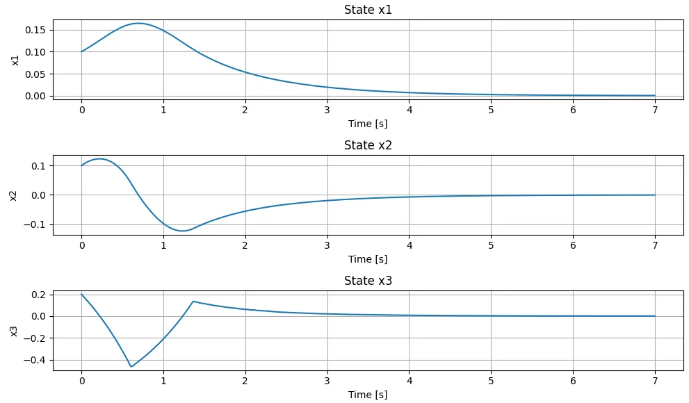
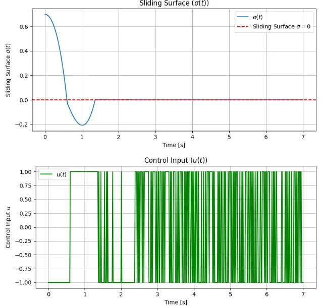
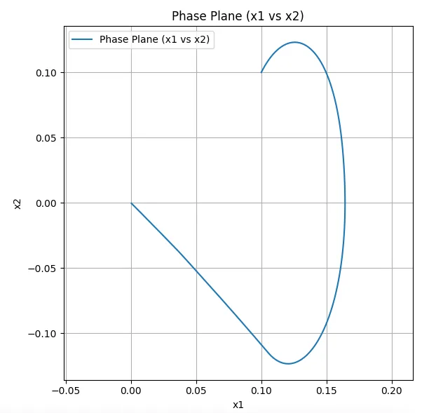
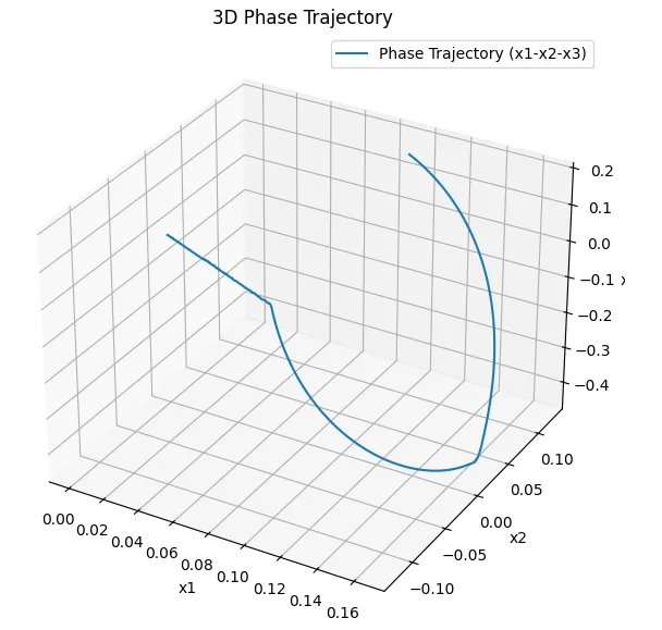
Pythonスクリプトとシミュレーション結果を示す。図１は、状態量$x_1,x_2,x_3$の時間応答である。全ての応答が0に収束している。図２は、スライディング面$\sigma$と制御入力の時間変化である。約1.3 sでスライディング面に到達し、スライディングモードで$[0,0,0]$に向かっている様子が分かる。図３は、状態量$x_1,x_2$による位相平面軌跡で$x_1=0.12,\;x_2=-0.12$において、スライディングモードに入っていることが分かる。図４は、状態量$x_1,x_2,x_3$の３次元位相軌跡で、スライディングモードで$[0,0,0]$に収束している様子がわかる。

import numpy as np
import matplotlib.pyplot as plt
from scipy.integrate import solve_ivp
from mpl_toolkits.mplot3d import Axes3D  # 3D plot support
# Define system parameters
a = 1.0  # Example value for 'a'
b = 1.0  # Example value for 'b'
# Given eigenvalues
lambda1 = -1
lambda2 = -2
# Compute k1, k2 from the given relationship
k1 = lambda1 * lambda2
k2 = -(lambda1 + lambda2)
# Define sliding surface S
S = np.array([k1, k2, 1])
# Define system matrices
A = np.array([[0, 1, 0],
              [0, 0, 1],
              [0, 0, a]])
B = np.array([[0], [0], [b]])
# Define the sliding mode dynamics
def smc_dynamics(t, x, A, B, S):
    # Sliding surface
    sigma = np.dot(S, x)  # スカラー値
    # Sliding mode control law
    u = -np.sign(sigma)  # スカラー制御入力
    # 状態方程式: dx = A*x + B*u（B: (3,1), u: スカラー）
    dx = A @ x + (B * u).flatten()
    return dx
# Initial condition for the state
x0 = np.array([0.1, 0.1, 0.2])  # Example initial state
# Time span for the simulation
t_span = [0, 10]
t_eval = np.linspace(t_span[0], t_span[1], 500)
# Solve the system with the sliding mode control
sol = solve_ivp(smc_dynamics, t_span, x0, args=(A, B, S), t_eval=t_eval)
# Plot the results: States
plt.figure(figsize=(10, 6))
plt.subplot(3, 1, 1)
plt.plot(sol.t, sol.y[0], label='x1')
plt.title('State x1')
plt.xlabel('Time [s]')
plt.ylabel('x1')
plt.grid(True)
plt.subplot(3, 1, 2)
plt.plot(sol.t, sol.y[1], label='x2')
plt.title('State x2')
plt.xlabel('Time [s]')
plt.ylabel('x2')
plt.grid(True)
plt.subplot(3, 1, 3)
plt.plot(sol.t, sol.y[2], label='x3')
plt.title('State x3')
plt.xlabel('Time [s]')
plt.ylabel('x3')
plt.grid(True)
plt.tight_layout()
plt.show()
# Calculate the Sliding Surface (sigma) for all time points
sigma_values = np.array([np.dot(S, sol.y[:, i]) for i in range(sol.y.shape[1])])
# Plot the Sliding Surface (sigma)
plt.figure(figsize=(8, 4))
plt.plot(sol.t, sigma_values, label='$\sigma(t)$')
plt.axhline(0, color='red', linestyle='--', label='Sliding Surface $\sigma=0$')
plt.title('Sliding Surface ($\sigma(t)$)')
plt.xlabel('Time [s]')
plt.ylabel('Sliding Surface $\sigma(t)$')
plt.grid(True)
plt.legend()
plt.tight_layout()
plt.show()
# Plot control input u
u_values = -np.sign(sigma_values)  # Control input based on the sliding surface
plt.figure(figsize=(8, 4))
plt.plot(sol.t, u_values, label='$u(t)$', color='green')
plt.title('Control Input ($u(t)$)')
plt.xlabel('Time [s]')
plt.ylabel('Control Input $u$')
plt.grid(True)
plt.legend()
plt.tight_layout()
plt.show()
# Phase plane plot (x1 vs x2)
plt.figure(figsize=(6, 6))
plt.plot(sol.y[0], sol.y[1], label='Phase Plane (x1 vs x2)')
plt.title('Phase Plane (x1 vs x2)')
plt.xlabel('x1')
plt.ylabel('x2')
plt.grid(True)
plt.axis('equal')
plt.legend()
plt.tight_layout()
plt.show()
# 3D Phase trajectory: x1 vs x2 vs x3
fig = plt.figure(figsize=(8, 6))
ax = fig.add_subplot(111, projection='3d')
ax.plot(sol.y[0], sol.y[1], sol.y[2], label='Phase Trajectory (x1-x2-x3)')
ax.set_title('3D Phase Trajectory')
ax.set_xlabel('x1')
ax.set_ylabel('x2')
ax.set_zlabel('x3')
ax.grid(True)
ax.legend()
plt.tight_layout()
plt.show()