6. スライディングモードのロバスト性

式(1)のシステムにおいて、$$\dot x = Ax + Bu,\quad \sigma = Sx \;\;\; \cdots (1)$$ 式(2)のように外乱の存在する系を考える。$$\dot x = Ax + Bu + h(x,t) \;\;\; \cdots (2)$$ここで、\(h(x,t)\)は、システムの不確かさと非線形性を含む関数とする。このとき、$$\dot \sigma = S\{Ax + Bu + h(x,t) \} = 0$$となるので、等価制御入力は、$$u_{eq} = -(SB)^{-1}S\{Ax + h(x,t)\}$$となる。スライディングモードが生じていれば、\(u_{eq}\)を式(2)に代入すると、$$\dot x = \{I - B(SB)^{-1}S\}Ax + \{I -B(SB)^{-1}S\}h(x,t) \;\;\; \cdots (3)$$となる。式(2)の系において、外乱\(h(x,t)\)が\(B\)のレンジスペースに存在するなら、$$h(x,t) = B \lambda(x,t) \;\;\; \cdots (4)$$と表現できる。
行列 \(B \in R^{n \times m}\)のレンジスペース（像空間）は、\(\text{Range}(B) = \{ y \in R^n \mid \exists\, \lambda \in R^m,\; y = B\lambda \}\)つまり、「行列\(B\)によって作れるベクトルの集合」である。ステムに作用する外乱 \(h(x,t) \in R^n\)が \(B\)の像空間にあるとは、 \(\exists\, \lambda(x,t) \in R^m\ \text{such that}\ h(x,t) = B\lambda(x,t)\)という意味である。つまり、外乱ベクトル\(h(x,t)\)は、行列\(B\)の列ベクトルによる線形結合として表現できる。つまり、外乱がレンジスペースにあることは、 外乱は「制御入力と同じ方向から入ってくる」ことなので、適切な制御入力で相殺できる可能性がある。
式(4)を式(3)に代入すると、スライディングモードが生じている限り、$$\dot x = \{I - B(SB)^{-1}S\}Ax + \{I - B(SB)^{-1}S\} h(x,t) \\ = \{I - B(SB)^{-1}S\}Ax + \{I - B(SB)^{-1}S\}B\lambda(x,t) \\ = \{I - B(SB)^{-1}S\}Ax + B\lambda(x,t) - B\lambda(x,t) \\ = \{I - B(SB)^{-1}S\}Ax \\ \sigma=0$$となり、外乱\(h(x,t)\)の影響は無くなる。

外乱の影響に関するシミュレーション例

$$\dot x = Ax+Bu, \quad \sigma=Sx$$のシステムに対して外乱が無い場合と外乱がある場合の応答に関してシミュレーションで確認する。
$$A=\begin{bmatrix} 0 & 1 \\ 0 & 0 \end{bmatrix}, \quad B=\begin{bmatrix} 0 \\ 1 \end{bmatrix} \\ S = \begin{bmatrix} 1 & 1 \end{bmatrix}$$とする。また、目標値は、\([x_1, x_2] = [1, \; 0]\)と単位ステップとする。初期値は、\([x_1, x_2] = [0, \; 0]\)である。外乱は、正弦波で\(h = B\cdot \sin(t)\)である。

Pythonスクリプトとシミュレーション結果を示す。
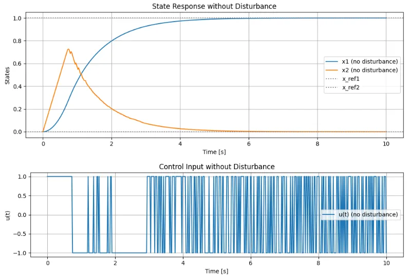
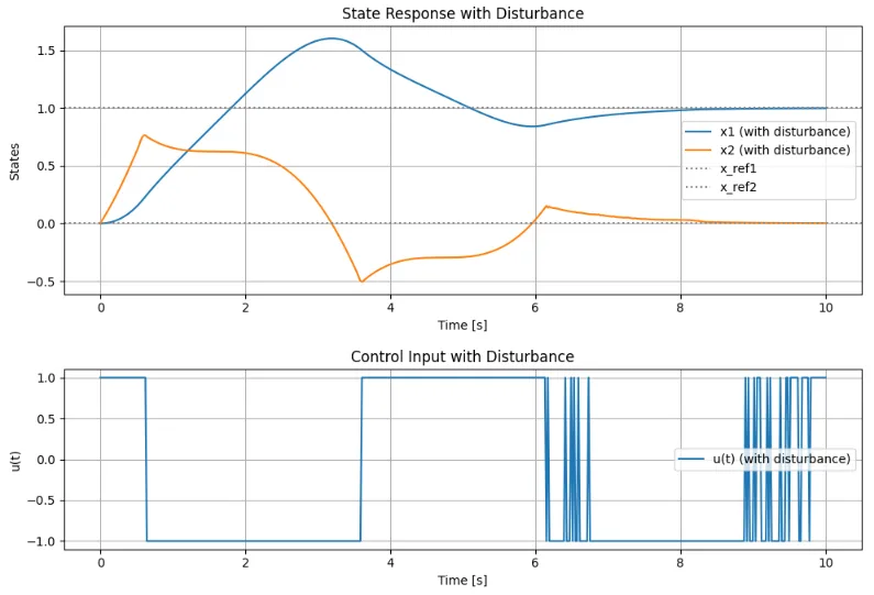
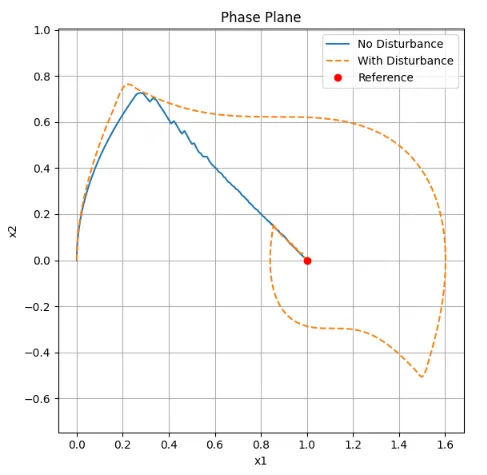
図１は、外乱が無い場合の状態量、制御入力の単位ステップ応答である。\([x_1,x_2]=[0.3,\;0.7]\)近傍でスライディング面に到達し、スライディングモードで目標値に到達している。　図２は、外乱が有る場合の状態量、制御入力の単位ステップ応答である。外乱（正弦波）により、状態量は大きく変動し、目標値に容易には近づけていない様子が分かる。しかし、図３（破線）から分かるようにスライディング面に到達した後は、スライディング面に拘束されてスライディングモードで目標値に達し、安定な状態を維持している。

import numpy as np
import matplotlib.pyplot as plt
from scipy.integrate import solve_ivp
# System matrices
A = np.array([[0, 1], [0, 0]])
B = np.array([[0], [1]])
C = np.array([[1, 1]])
S = C
x_ref = np.array([[1], [0]])
x0 = np.array([[0], [0]])
t_span = [0, 10]
t_eval = np.linspace(t_span[0], t_span[1], 500)
# Disturbance (B * sin(t))
def disturbance(t):
    return B @ np.array([[np.sin(t)]])
# SMC dynamics
def smc_dynamics(t, x, A, B, S, x_ref, disturb=False, phi=1.0):
    x = x.reshape(2, 1)
    sigma = S @ (x - x_ref)
    sigma_scalar = sigma[0, 0]
    if sigma_scalar > phi:
        u = -1.0
    elif sigma_scalar < -phi:
        u = 1.0
    else:
        u = -np.sign(sigma_scalar)
    h = disturbance(t) if disturb else np.zeros((2, 1))
    dx = A @ x + B @ np.array([[u]]) + h
    return dx.flatten()
# Simulate
sol_no_dist = solve_ivp(smc_dynamics, t_span, x0.flatten(), args=(A, B, S, x_ref,
False), t_eval=t_eval)
sol_with_dist = solve_ivp(smc_dynamics, t_span, x0.flatten(), args=(A, B, S, x_ref,
True), t_eval=t_eval)
# Control input trajectory
def control_input_traj(sol, A, B, S, x_ref, disturb=False):
    u_log = []
    for t, x in zip(sol.t, sol.y.T):
        x = x.reshape(2,1)
        sigma = S @ (x - x_ref)
        sigma_scalar = sigma[0,0]
        if sigma_scalar > 1.0:
            u = -1.0
        elif sigma_scalar < -1.0:
            u = 1.0
        else:
            u = -np.sign(sigma_scalar)
        u_log.append(u)
    return np.array(u_log)
u_no_dist = control_input_traj(sol_no_dist, A, B, S, x_ref, False)
u_with_dist = control_input_traj(sol_with_dist, A, B, S, x_ref, True)
# Plot: States without disturbance
plt.figure(figsize=(10, 4))
plt.plot(sol_no_dist.t, sol_no_dist.y[0], label='x1 (no disturbance)')
plt.plot(sol_no_dist.t, sol_no_dist.y[1], label='x2 (no disturbance)')
plt.axhline(x_ref[0, 0], color='gray', linestyle=':', label='x_ref1')
plt.axhline(x_ref[1, 0], color='gray', linestyle=':', label='x_ref2')
plt.title('State Response without Disturbance')
plt.xlabel('Time [s]')
plt.ylabel('States')
plt.grid()
plt.legend()
plt.tight_layout()
plt.show()
# Plot: Control without disturbance
plt.figure(figsize=(10, 3))
plt.plot(sol_no_dist.t, u_no_dist, label='u(t) (no disturbance)')
plt.title('Control Input without Disturbance')
plt.xlabel('Time [s]')
plt.ylabel('u(t)')
plt.grid()
plt.legend()
plt.tight_layout()
plt.show()
# Plot: States with disturbance
plt.figure(figsize=(10, 4))
plt.plot(sol_with_dist.t, sol_with_dist.y[0], label='x1 (with disturbance)')
plt.plot(sol_with_dist.t, sol_with_dist.y[1], label='x2 (with disturbance)')
plt.axhline(x_ref[0, 0], color='gray', linestyle=':', label='x_ref1')
plt.axhline(x_ref[1, 0], color='gray', linestyle=':', label='x_ref2')
plt.title('State Response with Disturbance')
plt.xlabel('Time [s]')
plt.ylabel('States')
plt.grid()
plt.legend()
plt.tight_layout()
plt.show()
# Plot: Control with disturbance
plt.figure(figsize=(10, 3))
plt.plot(sol_with_dist.t, u_with_dist, label='u(t) (with disturbance)')
plt.title('Control Input with Disturbance')
plt.xlabel('Time [s]')
plt.ylabel('u(t)')
plt.grid()
plt.legend()
plt.tight_layout()
plt.show()
# Plot: Phase Plane
plt.figure(figsize=(6, 6))
plt.plot(sol_no_dist.y[0], sol_no_dist.y[1], label='No Disturbance')
plt.plot(sol_with_dist.y[0], sol_with_dist.y[1], '--', label='With Disturbance')
plt.plot(x_ref[0], x_ref[1], 'ro', label='Reference')
plt.title('Phase Plane')
plt.xlabel('x1')
plt.ylabel('x2')
plt.grid()
plt.axis('equal')
plt.legend()
plt.tight_layout()
plt.show()