
5. スライディングモード制御の構造
スライディングモード制御は、線形制御とは異なり、線形制御系における状態方程式と出力方程式の対$$\dot x = Ax + Bu,\quad y = Cx + Du$$からなる状態空間モデルに代わって、状態方程式と切換関数の対からなるモデル$$ \dot x = Ax +Bu,\quad \sigma = Sx$$として表される。
スライディングモード制御系は、基本的に時間領域での設計、より厳密には位相空間での設計であるため、線形制御系のように時間領域、周波数領域と自在に変換して解析することができない。また、スライディングモード制御系は非線形制御系であるため、初期値によって特性が大きく異なる可能性があり、線形制御系のような周波数応答特性として制御性能を一般化して議論することができない。優れた性能が得られても、ある条件下でのことと捉えられることもある。これが非線形制御系の難しさでもある。
スライディングモードの存在条件
スライディングモードの存在条件1
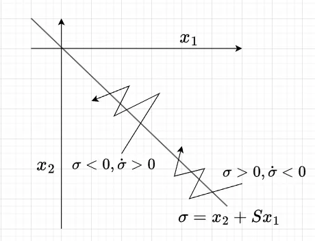
$$\begin{cases} \dot \sigma_i \lt 0 & if \quad \sigma_i \gt 0 \\ \dot \sigma_i \gt 0 & if \quad \sigma_i \lt 0 \end{cases} \;\;\; \cdots (1)\\ (i = 1, 2, \cdots, m)$$ 式(1)のとき、切換超平面\(\sigma_i =0\)の近傍でスライディングモード領域が存在する。図1は、1入力二次系\(i=1\)の例である。図のように\(\sigma = 0\)の両面で制御入力が切り換わりスライディングモードを生じる。システムは、任意の初期値から有限時間内に切換超平面およびその交線でスライディングモードを生じる。ただし、この条件は有限時間内に切換超平面に到達することは保証しない。
スライディングモードの存在条件2
この存在条件は、スライディングモード制御系の設計に良く使われる。
式(2)のリアプノフ関数を選定する。$$V = \frac{1}{2} \sigma^T \sigma \;\;\; \cdots (2) \\ \sigma(x) = [\sigma_1(x), \sigma_2(x), \cdots , \sigma_m(x)]^T$$式(2)の関数について、$$\dot{V}(\sigma) \lt 0$$を満足すれば、切換超平面\(\sigma_i = 0\)の近傍でスライディングモードが生じる。
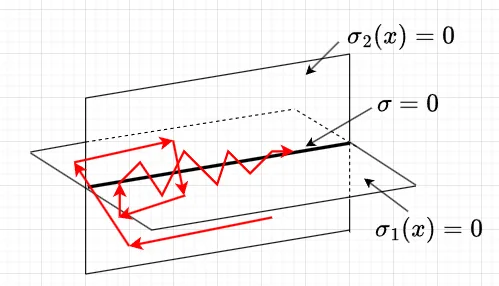
多入力系の場合、図2に示すように、各切換面\(\sigma_i = 0\)に達しただけではスライディングモードが生じず$$\sigma = [\sigma_1(x), \sigma_2(x), \cdots , \sigma_m(x)]^T=0$$つまり、各切換面の交線に収束して、初めてスライディングモードが生じる。より強い十分条件として、$$\dot V = \sigma \dot \sigma \lt - \eta|\sigma| \lt 0 ,\quad \eta \gt 0$$を満足すれば、全領域で切換超平面に到達できる。
等価制御法による解析
スライディングモードが存在する場合、システムは非線形性の強いスイッチング入力を必要とし、解析も困難となる。このスイッチング入力を等価な連続入力で置き換えることで、解析・設計の見通しが良くなる。これを等価制御と呼び、もとのシステムに代入力することで、スライディングモードにあるときのシステムの動特性を解析する。
システムを式(3)とする。$$\dot x = A x + Bu , \quad \sigma = S x \;\;\; \cdots (3)$$ \(B,\; S\)はフルランクとする。式(3)において、スライディングモードが存在すると、\(\dot \sigma =0\)である。従って、\(\sigma = Sx \)を時間微分すると、$$\dot \sigma = S \dot x$$となる。状態方程式\(\dot x = Ax + Bu\)を代入すると、$$\dot \sigma = S(Ax + Bu) = SAx + SB u$$スライディングモードでは\(\dot \sigma = 0\)であるため、$$SAx+SBu=0$$ここで、等価制御入力\(u_{eq}\)は、このスライディングモードを維持するために必要な制御入力である。従って、\(u\)を\(u_{eq}\)に置き換えると、$$SAx + SB u_{eq} = 0$$よって、$$SBu_{eq} = -SAx$$ \(B\)はフルランクであり、\(\det(SB) \neq 0\)ならば、\(SB\)の逆行列\((SB)^{-1}\)が存在するため、両辺に左から\((SB)^{-1}\)を掛けることで、等価制御入力\(u_{eq}\)が得られ、$$u_{eq} = -(SB)^{-1}SAx$$となる。この等価制御入力\(u_{eq}\)はシステムの理想的な連続制御入力である。\(u_{eq}\)を式(3)に代入すると、入力の数だけ低次元化されたシステムの式(4)が得られる。$$\dot x = \{I - B(SB)^{-1} S\}Ax \;\;\; \cdots (4)$$なお、導出過程から分かるように、この等価制御入力、及び、それによる低次元化されたシステムは、スライディング面に到達した後の等価的な制御システムである。スライディング面に到達するまでの制御入力は別に考える必要がある。
スイッチング入力と等価制御入力の比較
$$A = \begin{bmatrix} 0 & 1 \\ 0 & 0 \end{bmatrix}, \quad B = \begin{bmatrix} 0 \\ 1 \end{bmatrix}$$の線形時不変システムに対してスライディングモード制御によって目標状態 $$x_{ref} = [1, 0]^T \text{(= 単位ステップ)}$$へ状態を追従させる例を考える。スライディング面の定義は、 $$S = C(x - x_{ref})$$とする。
スライディングモードを適用したときのシミュレーションと等価制御入力(\(u_{eq} = -(SB)^{-1}SAX\))を適用としたときのシミュレーションを比較する。
Pythonスクリプトを以下に示す。
import numpy as np
import matplotlib.pyplot as plt
from scipy.integrate import solve_ivp
# システムパラメータ
A = np.array([[0, 1], [0, 0]])
B = np.array([[0], [1]])
# 目標状態
x_ref = np.array([[1], [0]])
# スライディング面パラメータ (Cは任意に設定)
C = np.array([[1, 1]])
S = C
# 初期状態(初期状態に大きく依存する)
x0 = np.array([[0.33], [0.68]])
# シミュレーション時間
t_span = [0, 10]
def sliding_mode_control(t, x, A, B, S, x_ref, phi=1.0):
"""スライディングモード制御"""
x = x.reshape(2, 1) # Reshape x to (2, 1)
sigma = S @ (x - x_ref)
# sigma is a (1,1) array, so extract the scalar value
sigma_scalar = sigma[0, 0]
if sigma_scalar > phi:
u = -1.0
elif sigma_scalar < -phi:
u = 1.0
else:
u = -np.sign(sigma_scalar)
# Reshape the result to (2,)
return (A @ x + B @ np.array([[u]])).flatten()
def equivalent_control(t, x, A, B, S, x_ref):
"""等価制御入力"""
x = x.reshape(2, 1) # Reshape x to (2, 1)
SA = S @ A
SB = S @ B
u_eq = -np.linalg.pinv(SB) @ SA @ x
# Reshape the result to (2,)
return (A @ x + B @ u_eq).flatten()
# スライディングモード制御のシミュレーション
sol_smc = solve_ivp(sliding_mode_control, t_span, x0.flatten(), args
(A, B, S, x_ref), dense_output=True)
# 等価制御入力によるシミュレーション
sol_eq = solve_ivp(equivalent_control, t_span, x0.flatten(), args=(A, B,
S, x_ref), dense_output=True)
# 時間軸
t = np.linspace(t_span[0], t_span[1], 100)
x_smc = sol_smc.sol(t)
x_eq = sol_eq.sol(t)
# スライディング関数
sigma_smc = S @ (x_smc - x_ref)
sigma_eq = S @ (x_eq - x_ref)
# 等価制御入力の計算
SA = S @ A
SB = S @ B
u_eq_sim = -np.linalg.pinv(SB) @ SA @ x_eq
plt.figure(figsize=(10, 8))
# 状態量のプロット
plt.subplot(3, 1, 1)
plt.plot(t, x_smc[0, :], label='$x_1$ (SMC)')
plt.plot(t, x_smc[1, :], label='$x_2$ (SMC)')
plt.plot(t, x_eq[0, :], label='$x_1$ (Equivalent Control)', linestyle='--')
plt.plot(t, x_eq[1, :], label='$x_2$ (Equivalent Control)', linestyle='--')
plt.plot(t, np.ones_like(t) * x_ref[0, 0], label='$x_{ref1}$', linestyle=':')
plt.plot(t, np.zeros_like(t) * x_ref[1, 0], label='$x_{ref2}$',
linestyle=':')
plt.xlabel('Time [s]')
plt.ylabel('State')
plt.title('State Trajectory')
plt.grid(True)
plt.legend()
# スライディング関数のプロット
plt.subplot(3, 1, 2)
plt.plot(t, sigma_smc.flatten(), label='$\sigma$ (SMC)')
plt.plot(t, sigma_eq.flatten(), label='$\sigma$ (Equivalent Control)',
linestyle='--')
plt.xlabel('Time [s]')
plt.ylabel('Sliding Function $\sigma$')
plt.title('Sliding Function')
plt.grid(True)
plt.legend()
# 制御入力のプロット
plt.subplot(3, 1, 3)
# The sliding_mode_control function returns a (2,) array.
# The list comprehension stacks these into a (100, 2) array.
# We only need the second element (index 1) for the control input.
u_smc = np.array([sliding_mode_control(ti, xi.reshape(2, 1), A, B, S,
x_ref) for ti, xi in zip(t, x_smc.T)])[:, 1]
plt.plot(t, u_smc, label='$u$ (SMC)')
plt.plot(t, u_eq_sim.flatten(), label='$u_{eq}$ (Equivalent Control)',
linestyle='--')
plt.xlabel('Time [s]')
plt.ylabel('Control Input $u$')
plt.title('Control Input')
plt.grid(True)
plt.legend()
plt.tight_layout()
plt.show()
# 位相平面図
plt.figure(figsize=(6, 6))
plt.plot(x_smc[0, :], x_smc[1, :], label='SMC Trajectory')
plt.plot(x_eq[0, :], x_eq[1, :], label='Equivalent Control Trajectory',
linestyle='--')
plt.plot(x_ref[0], x_ref[1], 'ro', label='Reference Point')
plt.xlabel('$x_1$')
plt.ylabel('$x_2$')
plt.title('Phase Plane')
plt.grid(True)
plt.legend()
plt.axis('equal') # スケールを同じにして見やすくする
plt.show()
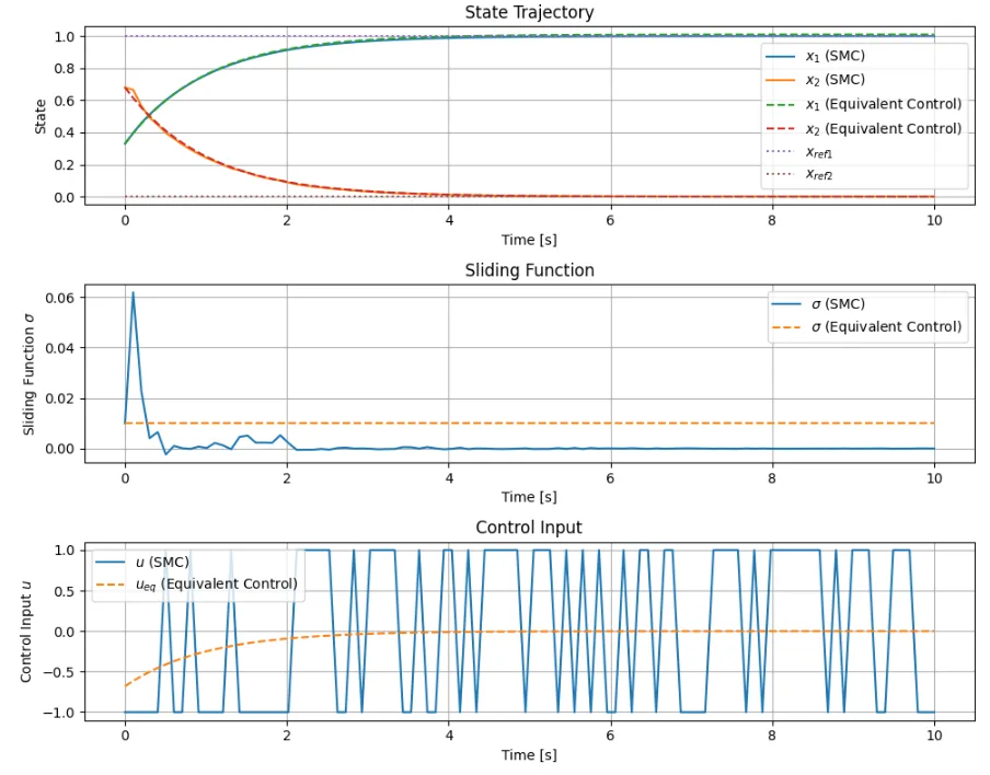
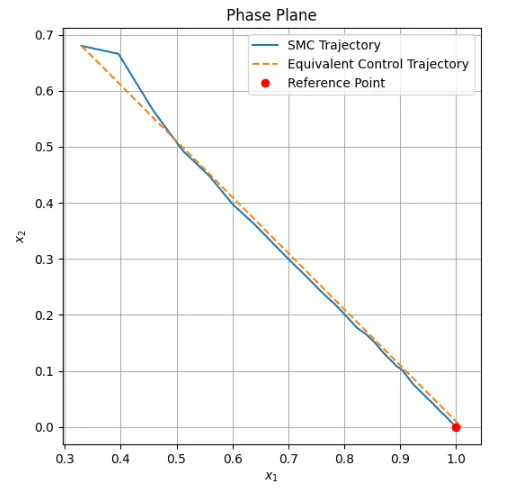
スイッチング入力と等価制御入力の比較では、当然のことながら初期値をスライディング面に到達した状態量に適切に設定しないと、等価制御のシミュレーション結果が大きくずれてくる。図3のように、スイッチング入力によるスライディングモード制御の制御量と等価制御入力による制御量の時間応答は、良い一致を示している。また、図3の制御入力の比較で分かるように等価制御入力は、スイッチング入力を積分したものとなっている。