17. 離散時間システムにおける状態推定(2)
まず、16. 離散時間システムにおける状態推定(1)の内容をまとめて示す。
離散時間システムとして、式(1)を考える。$$x_{k+1} = Ax_k + v_k \\ y_k = C x_k + e_k \;\;\; \cdots (1)$$ここで、\(v_k,\; e_k\)は平均値0の正規白色雑音でそれぞれの分散を\(R_v,\; R_e\)とする。また、初期状態\(x_0\)の平均値を\(m\) 、分散を\(R_0\)とする。状態推定器は式(2)とする。$$\hat{x}_{k+1} = A \hat{x}_k + K_k (y_k - C\hat{x}_k) , \quad \hat{x}_0 = m \;\;\; \cdots (2)$$これを使って、式(1)の状態変数を推定する。2乗平均の意味において最適な推定解を得るには、ゲイン行列\(K_k\)を式(3)のように決定する。$$K_k = A P_k C^T(R_e + C P_k C^T)^{-1} \;\;\; \cdots (3)$$また、\(P_k\)は推定誤差の共分散で式(4)で与えられる。$$P_{k+1} = A P_K P^T + R_v - A P_k C^T(R_e + C P_k C^T)^{-1} C P_k A^T \;\;\; \cdots (4) \\ P_0 = R_0$$共分散\(P_k\)は、観測値に依存しないので、\(P_k,\; K_k\)は予め計算しておくことができる。よって、最適フィルタをオンラインで計算実行する場合、\(P_k,\;K_k\)は予め計算して記憶しておけばよい。
17-1. カルマンフィルタによる状態推定
サンプリング周期\(T = 0.01\)[s]で離散化したシステムを式(5)とする。$$x_{k+1} = \begin{bmatrix} 0.995 & 0.009 \\ -0.993 & 0.985 \end{bmatrix} x_k + v_k \\ y_k = \begin{bmatrix} 1 & 0 \end{bmatrix} x_k + e_k \\ x_0 = \begin{bmatrix} 10 \\10 \end{bmatrix} \;\;\;\quad \quad \cdots(5)$$また、システム雑音、観測雑音の平均値と分散を式(6)とする。$$E[v_k]=0, \quad E[v_k v_k^T]=\begin{bmatrix} 0.3 & 0 \\ 0 & 0.8 \end{bmatrix} \\ E[e_k] = 0, \quad E[e_k e_k^T] = 0.4 \;\;\; \quad \quad \cdots (6)$$このときの状態推定の振る舞いを求める。
状態推定器の初期値\(\hat{x}_0\)と推定誤差分散の初期値\(P_0\)を以下の値として、式(5)の離散時間システムの状態量\(x_1,\; x_2\)とそれぞれの推定値\(\hat{x}_1,\; \hat{x}_2\)の時間応答を計算する。$$\hat{x}_0 = \begin{bmatrix} 10 \\ 10 \end{bmatrix} , \quad P_0 = \begin{bmatrix} 0 & 0 \\ 0 & 0 \end{bmatrix}$$
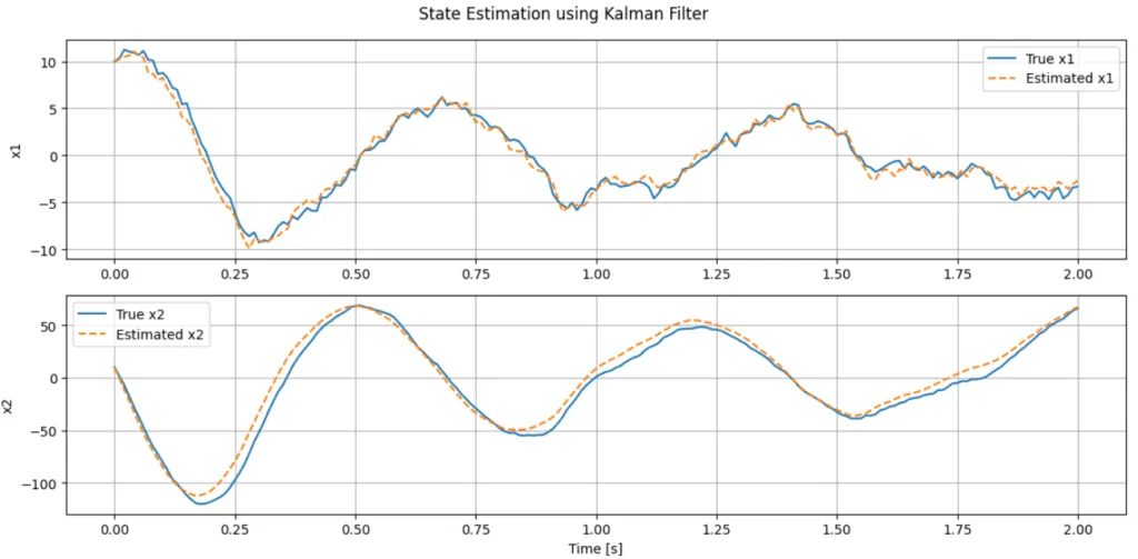
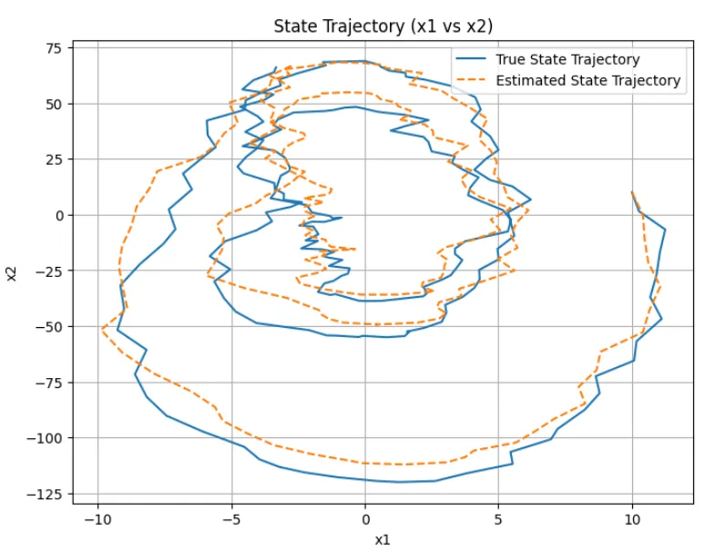
※Pythonのスクリプトは、以下のようになる。また、図1、図2に実行結果を示す。図より、状態を上手く推定できることが分かる。
import numpy as np
import matplotlib.pyplot as plt
# System parameters
T = 0.01 # Sampling period
A = np.array([[0.995, 0.009],
[-0.993, 0.985]])
C = np.array([[1, 0]])
# Noise characteristics
Rv = np.array([[0.3, 0],
[0, 0.8]]) # Process noise covariance
Re = np.array([[0.4]]) # Measurement noise covariance
# Initial conditions
x0 = np.array([[10],
[10]]) # True initial state
x_hat0 = np.array([[10],
[10]]) # Initial estimated state
P0 = np.array([[0, 0],
[0, 0]]) # Initial estimation error covariance
# Simulation settings
N = 200 # Number of time steps
x = np.zeros((2, N+1))
x_hat = np.zeros((2, N+1))
y = np.zeros((1, N+1))
# Initialization
x[:, [0]] = x0
x_hat[:, [0]] = x_hat0
P = P0
# Random seed for reproducibility
np.random.seed(0)
# Kalman filter simulation
for k in range(N):
# Generate process and measurement noise
v_k = np.random.multivariate_normal(mean=[0, 0], cov=Rv).reshape(-1, 1)
e_k = np.random.normal(loc=0, scale=np.sqrt(Re)).reshape(1, 1)
# System update (true state)
x[:, [k+1]] = A @ x[:, [k]] + v_k
# Measurement
y[:, [k+1]] = C @ x[:, [k+1]] + e_k
# Prediction step
x_pred = x_hat[:, [k]]
P_pred = A @ P @ A.T + Rv
# Kalman gain
K = A @ P_pred @ C.T @ np.linalg.inv(C @ P_pred @ C.T + Re)
# Update step
x_hat[:, [k+1]] = A @ x_pred + K @ (y[:, [k+1]] - C @ x_pred)
P = P_pred - K @ C @ P_pred @ A.T
# Time vector
time = np.linspace(0, T*N, N+1)
# Plotting results
plt.figure(figsize=(12, 6))
plt.subplot(2, 1, 1)
plt.plot(time, x[0, :], label='True x1')
plt.plot(time, x_hat[0, :], label='Estimated x1', linestyle='--')
plt.ylabel('x1')
plt.legend()
plt.grid()
plt.subplot(2, 1, 2)
plt.plot(time, x[1, :], label='True x2')
plt.plot(time, x_hat[1, :], label='Estimated x2', linestyle='--')
plt.xlabel('Time [s]')
plt.ylabel('x2')
plt.legend()
plt.grid()
plt.suptitle('State Estimation using Kalman Filter')
plt.tight_layout()
plt.show()
# Plot x1 vs x2
plt.figure(figsize=(8, 6))
plt.plot(x[0, :], x[1, :], label='True State Trajectory')
plt.plot(x_hat[0, :], x_hat[1, :], label='Estimated State Trajectory', linestyle='--')
plt.xlabel('x1')
plt.ylabel('x2')
plt.title('State Trajectory (x1 vs x2)')
plt.legend()
plt.grid(True)
plt.show()